ADAM Technology Team Blog

I have uploaded a video to our YouTube channel that illustrates how to use UAVs with our software. (Be sure to change the video quality to 720p if you have a good Internet connection!) In this post I’d like to cover the topic in more detail than the video and accompanying description allows.

UAVs

ADAM Technology has been involved with using and optimising Unmanned Aerial Vehicles (UAVs), also known as Unmanned Aerial Systems (UASs), for aerial photography since 2006.

During this time UAVs have evolved from R&D prototypes into a valuable surveying and mapping tool. The design of the A.I.Tech 880MX shown in the video, for example, takes into account the experience gained over that time, and features dual-redundant down links operating at different frequencies with automatic failover in the case of a loss of communication on one link; the ability to conduct an entire flight fully autonomously, including landing; a flybarless head design for added efficiency; and well over a hundred hours of flawless operation producing data just like that shown in the video (which, in fact, was just one project from 11 that it flies every month at one customer’s site).

Since we’re planning to use the images for photogrammetry, all we really care about is getting a camera into the right locations to capture good images of the scene. UAVs have many highly desirable characteristics from that point of view:

1. Being an aerial platform, they can achieve the perfect vantage point for a number of important applications, including stockpile volumes.

2. Being autonomous with on-board GPS, they reliably and repeatedly produce images with the correct separation along straight flight lines at the correct distance.

3. For areas up to about 10 km², the speed with which they can capture that area at that level of detail and accuracy is difficult to match with any other technology. (Conventional aircraft with large format cameras can cover larger areas even faster, and are a good option when larger areas need to be captured, but they have lower limits on detail and accuracy that a UAV can easily exceed, and because they fly higher they are also more affected by cloud cover.)

(Click here if the video does not appear above.)

UAVs could also conceivably be used with other remote sensing technologies, like LIDAR; however, the huge advantage of using them for photogrammetry instead is that a digital camera is an extremely cheap and light-weight payload compared to a laser scanner and associated IMU; this means a cheaper and lighter UAV can be used to produce more accurate and denser data, and if something goes wrong the financial consequences are far less serious.

In addition to conventional cameras, at least one customer has used a thermal camera in conjunction with our software and a UAV to map hot spots in a sensitive area.

Aerial Photography

As explained in my earlier Blog post on aerial photography, and illustrated in the video, images typically overlap by 60% within the same strip and about 25% between strips. This allows the software to tie the entire project together, sharing control, and to make sure every point on the surface appears in at least two images so that a 3D location can be determined for that point. However, since taking a picture is essentially free with a digital camera, we actually capture images with an 80% overlap, i.e. we capture images twice as often:

This gives us a few options:

1. If an image doesn’t turn out, it doesn’t mean we end up with a hole in our data — we simply switch to the neighbouring image instead and continue on. (So if there was a problem with image 5 in the sequence 1-3-5-7-9, we could instead use 1-3-4-6-8-10.) With an 80% overlap, two images in a row would have to be unusable before we actually had a problem; this is so rare that we accept that risk, but if it was common enough to be worth the effort, we could increase the overlap to 90% — again doubling the capture frequency — and then four images in a row would have to be bad before it affected our ability to generate data for a particular location.

2. If we want more detail and accuracy (and an improved ability to see beneath infrastructure like conveyor belts, for example) then we can actually process all images at a cost of longer processing times. In the case of the project on the video, using all images instead of every second image results in over 20 million points in total — more than 50 points per square metre. In this case, bad images will result in areas of lower density (i.e. the same density as we would get by just processing every second image to begin with).

3. If we want to double-check the accuracy of our data, we can process the two sets of images independently and then compare their DTMs. In the case of the project on the video, comparing the final surface models generated by all the even-numbered images vs all the odd-numbered images revealed a mean difference of 3.6 cm, well within our stated accuracy of 5 cm.

Control

I have briefly referred to control points before, in “How Does Photogrammetry Work?”, “How Accurate is Photogrammetry? — Part 3”, and “Residuals”, but I should probably explain them in a little more detail.

In our software, two types of points are used:

• Relative-Only Points, also known as “tie points”, are points that are in two or more images that (should) correspond to the same location in the scene that we don’t already have 3D locations for; and

• Control Points, which are points that are in one or more images that we do have 3D location information for in advance, typically by surveying with GPS, a total station, or even a previous 3DM Analyst Mine Mapping Suite project.

Relative-only points, which are normally generated automatically by the software (as shown in the video) by simply looking for common points between images, are useful for figuring out where the cameras are in relation to each other and what direction they are pointing in — their relative orientation. The Free Network Resection and Bundle Adjustment use the image co-ordinates of those relative-only points — and nothing else — to establish that relative orientation. (Step 3 in the video.) Once the relative orientation has been determined, 3D co-ordinates for all of those points are calculated, and that is what is shown in the 3D View just after the 3 minute mark in the video.

As explained in my post on residuals, once 3D co-ordinates have been determined, the software can project those 3D co-ordinates back onto the original images and compare the image co-ordinates derived from those 3D co-ordinates with the image co-ordinates that were originally determined by the matching process. If a small number of points have large residuals, it suggests that the points did not actually correspond to the same location in the scene and so we call those “bad points”; the software can actually remove those bad points itself, automatically, which you can see at the 2:40 mark in the video — in other words, not only does the software generate all the information it needs to in order to establish the relative orientation itself, it can even detect when it’s made a mistake and clean it up!

While all of this is welcome indeed, in practice we often want the data to be established in some particular co-ordinate system; it’s no use having a wonderful, detailed surface model of a stockpile or pit if we can’t relate it to the real world. A street directory for New York is not useful if you’re trying to get around Sydney. (This is not always the case; for example, a 3D model of an ancient Roman coin does not need to be in Universal Transverse Mercator, and it would be odd if it was because it would be wrong as soon as you picked it up. In that case you really do want an arbitrary co-ordinate system, probably centred on the object itself, and with scale the only important real-world component. If you look at the Free Network dialog in the video you can see how the co-ordinate system for a relative orientation can be customised.)

The most common way of establishing a real-world co-ordinate system is by providing the software with the 3D co-ordinates (in the desired real-world co-ordinate system) of points that are visible in the scene. Mathematically we need three such points that are not in a straight line; for this reason, in the video, I digitised three control points (1, 3, and 6) before calculating the absolute orientation. Once the absolute orientation has been determined, the software knows where to look in the images for any remaining control and we can use the “Driveback” feature to automatically digitise them (4:12 in the video) if circular targets were used. We incorporate these additional control points into the absolute orientation by repeating the Bundle Adjustment and then examine the residuals of the control points for an indication of the project’s accuracy. (Note that at 4:09 we already have residuals using the three control points digitised at that point; these residuals are worthless for estimating accuracy, however — note the height residual of 1 mm! — because with only three points there is very little redundancy, and entire classes of errors would be completely invisible to the software. Being able to detect bad control and being able to estimate accuracy from the control point residuals are two of the main reasons for using more than three control points. The other reason is to improve accuracy, because the more observations you have, the more accurate the results will be.)

Placement

Control points should, ideally, bracket the area of interest. This is because the further we venture from the area surrounded by control points, the more any error in those control points is exaggerated. Interpolation between control points will be more accurate than extrapolating beyond the control points. Placing all of the control points close together in one corner of the project will greatly diminish the value of those control points.

Note that the three control points I chose to digitise in the beginning (1, 3, and 6) also happened to be widely dispersed. This gave an initial exterior orientation that was accurate enough that the remaining points could be picked up successfully.

Design

In the video, circular targets were used as control points:

These have the advantage that the software can automatically find their centre very accurately (better than 0.1 pixels), provided the user either clicks in the vicinity (first three control points) or the software can predict their locations (remaining control points). If the control points are semi-permanent (as these are — note the star pickets holding the control point in place) then the effort to create them can be worthwhile.

But other designs can be used as well:

The underground projects YouTube video shows how control points can be digitised by hand, and although it’s certainly less convenient, it would have added only about one minute to the time required to complete this project.

Camera Stations

Yet another option, used when control points are impossible or even merely inconvenient, is to use the UAV’s onboard GPS to record camera positions directly. There are disadvantages:

1. Conventional GPS is normally used for UAV navigation because its accuracy is perfectly fine for following flight lines to the required accuracy for aerial photography; for camera locations, however, differential GPS would normally be required to get close to the accuracy possible with ground control, adding expense.

2. Because the aircraft is in motion, differential GPS will still normally be not as accurate as differential GPS on the ground.

3. Errors can be harder to detect.

On the other hand, it’s certainly very convenient to simply fly a project and not have to place and survey control points at all, so there is a strong desire to do this; as a consequence, we recently added the ability to batch-import camera stations to use as part of the exterior orientations and will continue to refine this workflow.

Workflow

The workflow being followed features prominently throughout the video. In particular it is worth noting that control points are used to determine absolute orientations quite early on, before any DTMs have been generated. Not all systems work this way — some actually generate the DTMs using the relative orientations (so the DTMs are in an arbitrary co-ordinate system) and then convert the data into the desired co-ordinate system by digitising the control points on the DTMs and performing a Helmert transformation (i.e. translation, scale, and rotation) to georeference the data.

This is not the best practice for a couple of reasons:

1. Using the control points to construct a Helmert transformation after the data has already been generated removes any possibility of the control point information being used as an input to the bundle adjustment to improve the accuracy of the orientations. All inputs have errors, including the relative-only point locations and the camera calibration, and using all available information — which includes control point locations and their associated accuracies — means the optimal solution can be found. Separating the absolute orientation into two steps — a relative orientation followed by a Helmert transformation — prevents this.

2. The accuracy with which points can be digitised on a point cloud/DTM is far lower than the accuracy with which points can be digitised in an image, mostly because the point cloud is a lot sparser than the image pixels. It’s also more difficult and error-prone. This, in turn, lowers the accuracy of the georeferencing. As mentioned before, our software’s automatic circular target centroiding is accurate to better than 0.1 pixels, and the typical manual control point digitising accuracy is about 0.2 pixels.

3. Any problems with the control points are identified early on, before too much effort has been expended.

Other Examples

Here is a surface model and oblique orthomosaic of a stockpile generated from images captured by a customer in the US using a UAV:

That particular project area was about 300 m x 365 m and was captured with 37 images in 9 minutes from an altitude of 115 m. It takes 14.5 minutes to process the images and generate over 9 million points.

Below is part of the actual DTM of the pit that we generated with the prototype UAV in the first image:

That DTM consists of 2.3 million points generated from ten images and took 7 minutes to process. An orthophotomosaic can be downloaded from here and an image of the contours from here. The launch site (where the first image above was captured) is the raised area on the upper-right with the two lumps in it (from the two vehicles).

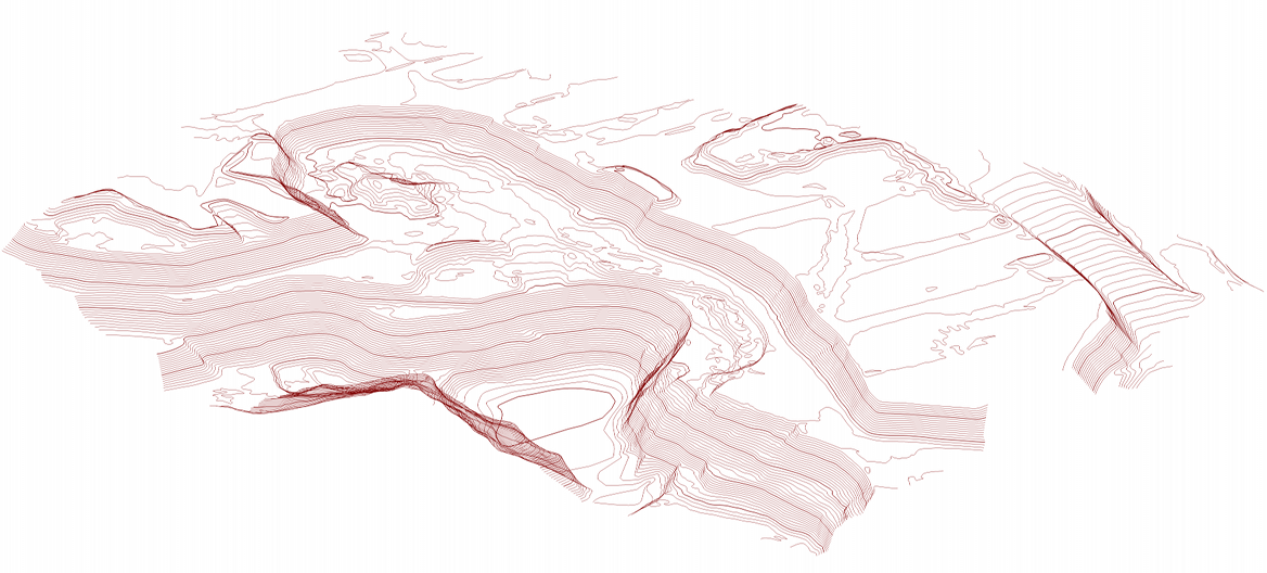
The area was about 300 m x 200 m and the height variation was about 35 m. The point density was about 40 points per square metre, or about one point every 15 cm.

Subsidence monitoring is another interesting application area:

It took 17 minutes of flying to capture the 630 m x 440 m area and about 1 hour of processing to generate 29 million points.

Conclusion

After several years of refinement UAVs have now proven themselves extremely valuable for an important range of applications. Coupled with our software they make an extremely attractive option indeed!