It’s been a while! Time flies when you’re having fun. Anyway, I thought this would be a good topic to discuss because many people don’t really understand what residuals are and most people don’t make as much use of them as they could.
What are residuals?
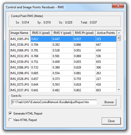
They show up in our software in quite a few places, such as the control (“Control Point RMS”) and image points (“RMS X”, “RMS Y”, “RMS Pt”) residuals in the control network bundle adjustment results dialog in 3DM CalibCam:
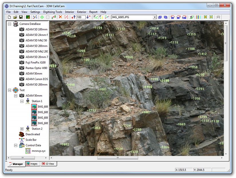
They’re also depicted as little tails on each point in the Images View, with the tail representing both the direction and the magnitude:
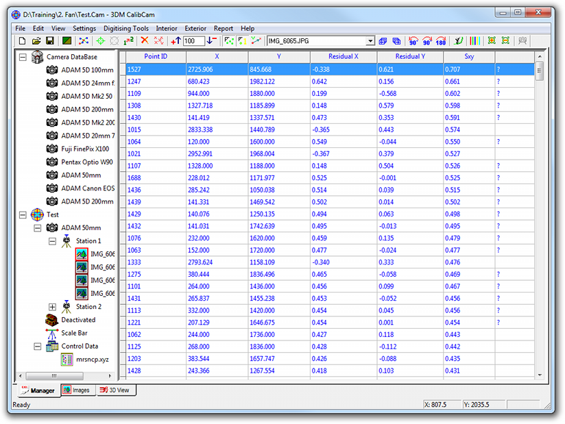
And numerically (conveniently sorted by size, so the worst offenders appear at the top) if you click on the “Toggle Image Display” button in the toolbar:
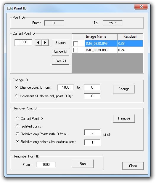
You can even remove points based on their residuals automatically, using the Edit | Remove Bad Relative-Only Points menu, or manually, using the Edit Point IDs dialog:
Clearly they must be important. But what are they, and what do they tell us?
Background
Let’s take a step back for a moment and think about a simple problem so that the concepts become clearer.
Suppose we had some physical process that we could observe and measure, and suppose that we wanted to understand that physical process well enough to predict what measurements we are likely to get in the future.
How are we going to do that?
The first thing we need to do is propose a model — a mathematical representation — for that physical process. (Ideally, we should have some reason for believing the model to be appropriate, but fortunately we can usually tell if it’s not.)
Now, many models have parameters that we can tune, so next we need to take some observations and try to fit the model to them — that is, determine the correct values for the various parameters in the model, preferably in a way that allows us to detect if the model is actually correct or not (i.e. whether our original belief was justified) and even whether the model is overly complicated (i.e. some of the parameters are redundant and can be removed).
This is complicated slightly by the fact that real-world observations will have errors, and so therefore our model will never perfectly fit the data, even if the model is actually correct.
To explore these ideas I have created a spreadsheet that you can download from our website to play with:
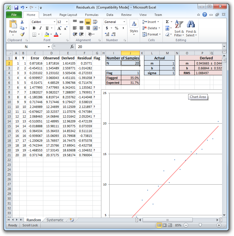
The model we are going to try fitting in this case is a linear function of the form y = mx + b, where m and b are the parameters. This is convenient because not only is it simple to understand, Excel also includes a function to do the hard work for us, although it’s not hard to code it up by hand.
To generate data the spreadsheet helpfully uses a linear function of the form y = mx + b, so we do have a good reason for believing a linear function will work in this case. 🙂
To make things interesting, however, the spreadsheet will add random noise to the “true” Y values in order to simulate real-world observations with errors.
So, in the spreadsheet, the first column “X” represents the independent variable and the second column “Y” represents the true value of the quantity being observed. (If you want a real-life physical process that we could be measuring, a bathtub filling with water from a tap flowing (or dipping) constantly would be one. In that case, X would be time and Y would be depth.)
The third column, “Error”, is the normally-distributed random error added to each observation. The magnitude of that error is controlled by the “sigma” value in M4. Increase sigma to make the observations more noisy, reduce it to make them more accurate.
The fourth column, “Observed”, is what we actually see when we make the measurements. Note that we don’t know what the true value of Y is, and we don’t know what sigma is — all we know at this stage are the observations. We need modelling to derive both the true values of Y and an estimate of sigma.
Under “Number of Samples” you can enter a value between 1 and 1000 and the spreadsheet will automatically generate that many observations for you. It’s a good idea to play with this because you’ll quickly discover that when the number of observations is low and the error is high, the parameter estimation for our model is not terribly good — this is why it’s a good idea to have lots of redundancy. Set N to 1000 and the estimates should become very good indeed.
Under “Actual” you can set the actual, underlying process and, as mentioned above, the accuracy of the observations. Experiment with setting m, b, and sigma to any values you want.
The next table, “Derived” shows what Excel deduced the values of m, b, and sigma to be, as well as how accurately it thinks the estimate of m and b is. (I’ll come back to “RMS” in a minute.)
(The final table is just a cheat to get the modelled slope plotted on the graph — since it’s a straight line, we only need the two endpoints to plot it. We could use Excel’s ability to plot a trendline to get the same thing but I wanted to make it explicit.)
OK, so the Derived table shows what Excel thinks m and b are, while the Actual table shows what they really are. We can see how good the Derived values are by calculating, for each X, what we think the Y value should have been. That’s what the Derived column is, column E in the spreadsheet. That column is using our model to predict what the true value of Y should be, without the observation error.
If we then compare the observed value with the derived value, we get column F — the Residual!
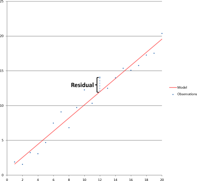
So, the residual is nothing more than the difference between what our model predicts a particular observation should be and what we actually observed. In the graph, it’s the vertical difference between the blue dot of a particular observation and the red line. LINEST finds the values for m and b that minimises the sum of the squares of the residuals — that is, if you squared each residual, and added them all up, then any other value you cared to try for m and b would result in a larger number.
Why is this useful?
Well, suppose that we got the model itself correct, and we estimated the parameters of that model correctly. That means that the residuals themselves are exactly the same as the error we added to the true values to determine the observations! Which means that if we compute the standard error, or RMS (Root-Mean-Squared) of the residuals, we are actually calculating the magnitude of the observational error! This is what the RMS field of the Derived table is doing. Provided there are enough observations, the RMS value should be almost the same as the sigma value, because in this particular spreadsheet we have got the model correct (by construction) and we are estimating the parameters optimally (using a least squares best fit, which is what Excel is doing internally).
So, not only can we parameterise our model from noisy observations, we can even tell how accurate the original observations were! Indeed, when checking the results of a bundle adjustment, it’s a good idea to verify that (1) the image points RMS values are similar to the expected image accuracy for that camera and lens, and (2) the control points RMS values are similar to the supplied accuracy specifications. If they are much larger, that’s a sign something is wrong. (If they are much smaller then that’s a sign something might be wrong, also. If it’s the image points RMS values then you may have accidentally removed “good” points by using the Edit Point IDs dialog to remove points with residuals above a low value; if it’s the control points RMS values then you may not have enough control points or their geometry may be too poor for the residuals to be a reliable indicator of accuracy.)
What else can we do?
Well, there’s another table and column that hasn’t been explained yet: “Flag”. The “Flag” value in J4 is used by the “Flag” column to highlight suspicious observations, by checking to see how many multiples of the derived RMS is that particular observation’s residual. If an observation’s residual is more than Flag x RMS, it gets a question mark next to it. (Note that you can see a similar question mark in the 3DM CalibCam screenshot showing the residuals table as well; in this case, the Flag value is hardwired to 3 × the specified accuracy.)
The next entry in the Flag table is the percentage of observations that were flagged using that particular flag setting.
The final entry in the Flag table is the percentage of observations that we would expect to be flagged using that particular flag setting if the observations are subject solely to normally-distributed random errors. (This is a subtle but important point — the nature of our observation errors was also a model!)
This last point is important to understand — if errors are normally distributed, and we have correctly determined the standard deviation of the observational error, then we expect about 32% of the observations to have errors larger than one standard deviation! We also expect about 4.6% to have errors larger than two standard deviations. (We also expect about 5% to have errors larger than 1.96 standard deviations.)
What about three standard deviations? That turns out to be about 0.3% of observations, or three per thousand observations can “legitimately” have errors larger than 3 × sigma. More on that shortly.
How is this useful? Well, if an observation has a large enough residual in terms of number-of-standard-deviations, we can conclude that it’s sufficiently unlikely to have occurred purely by chance that it must be a “blunder”, as opposed to normal observation error. Why? Because either a gross error was made, or our model of the observation errors is wrong, and we have really good reasons for assuming a normal distribution for random observation error (see “Central Limit Theorem” for why).
So what could cause this? If it’s in the surveyed ground co-ordinates, it could be an instrument error, operator error, or software user error where the point was mis-identified. I once did a trial where three of the 15 control points supplied were “blunders”, one of them 2 km away from where it was supposed to be! That one turned out to be a fit of dyslexia on the part of the surveyor, transposing two digits in the co-ordinates when transferring it to the PC by hand. For relative-only points, it’s most likely to be a mismatched point. In fact, the menu Edit | Remove Bad Relative-Only Points looks at each image in turn, derives the average RMS for that image, and then removes any points with residuals more than three times greater than that, on the basis that such an error is pretty unlikely if the point only has random error.
So, looking at residuals and comparing them to the RMS allows us to quickly identify points that are likely to be blunders. It’s important to get rid of those points because one of the guarantees that the bundle adjustment makes — that the result is the optimal one — only holds true if the observation errors are normally distributed. Blunders cause the residuals to have fatter tails than they should — i.e. the distribution of residuals is not perfectly normal. Think about that off-by-2-km control point — given a survey accuracy of 0.1 m, that represents an error of 20,000 × sigma — something that should simply never happen. And yet it did. So we need to filter out those points if we are to obtain the optimal results.
You can test the “blunder detector” by manually overwriting a value in the Observations column with something absurd. Provided there aren’t too many of them relative to the overall number of observations, and Flag is set to a reasonable value (like 3), it should reliably detect your bad observations (and, despite my warnings, should not have too great an impact on the derived m and b values unless N is small).
What else can residuals tell us?
Apart from blunders, there is one other way that residuals can be non-normally distributed. What if the model is actually wrong? In our spreadsheet we used a simple linear function. If, instead, we used a quadratic to generate the values but continued to use a linear function to model the values, the residuals would not only contain random errors — they’d contain systematic errors as well!
You can click on the Systematic tab of the spreadsheet to see an example of exactly this — now the actual underlying function is y = ax2 + bx + c, but we’re still trying to fit a linear function to it of the form y = mx + b. (If you set a to 0 in cell M2 then you’ll see everything still works.)
So how do we recognise when this is occurring? There are two ways. Firstly, the residuals are large relative to the expected observational accuracy. (In the example figure below, the observed RMS is about 30 times larger than sigma. Increase the number of points beyond 20 and the observed RMS becomes truly enormous due to the effect of the x2 term.) For image co-ordinate residuals, the expected accuracy is the image sigma that we determined during calibration. For control point residuals, the expected accuracy is the surveyor-supplied accuracy. If the model is wrong, the RMS’s of the residuals will not be consistent with what we expected — generally much higher.
Secondly, you will normally find a pattern to the residuals. Look at the Excel graph again — notice how nearby points have very similar residuals, both in magnitude and direction? There is a lot of correlation between nearby residuals — this is a key indicator of a systematic error. By contrast, when we are dealing with purely random error, the neighbouring residuals are uncorrelated.
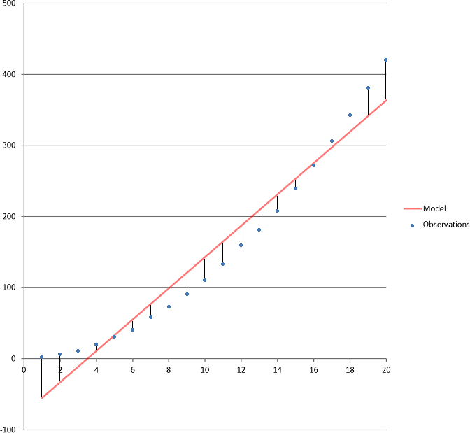
Note that there is nothing to stop us from using a quadratic function as our model and attempting to use LINEST to determine the best parameters for that model — the term “linear” in the phrase “linear regression” (which is what we’re using) does not refer to the model, which just happened to be linear in the first example, but rather that our best fit is a linear function of the input data. For example, ax2 + bx + c is a linear function of x2 and x with parameters a, b, and c.
Real-life examples
OK, so hopefully we now have a better idea of what residuals actually are, and also understand how we can use them to (a) detect blunders and (b) detect systematic errors (i.e. an incorrect model). It’s time to start thinking about how this applies to our software in concrete terms.
What is the model? Your first answer would probably be “the camera calibration”, and you’d be right, that is one of them — when we calibrate a camera, we are implicitly assuming that the real-world camera’s behaviour is accurately characterised by the software’s internal model of a camera, and there are several ways in which that model could be wrong. But there are other models as well — for example, if you place multiple images on the same camera station, and tell the software that the camera station is a “No Offset” camera station, then you are invoking a model that says each of those images has a common perspective centre, and that can be wrong as well!
Before delving into the details, however, it’s probably worth looking at how the residuals are actually calculated. For image co-ordinate residuals, the derived 3D co-ordinates of all of the control points and relative-only points are projected back onto the images, using the derived exterior orientations, to generated adjusted image co-ordinates. The image points residuals then are simply the differences between these derived image co-ordinates and the observed image co-ordinates. For the control point residuals, the same thing applies — the derived 3D co-ordinates of the control points are compared to the supplied 3D co-ordinates. (Note that the bundle adjustment simultaneously determines both the 3D co-ordinates for all of those points and the exterior orientations such that the residuals of the image co-ordinates and ground co-ordinates are minimised according to their specified accuracies.)
So let’s look at each of the things in the real world that can invalidate the various models that the software uses, and how we might detect those.
-
Mixing up the camera calibrations and choosing the wrong one for the project. This will normally present itself as large residuals with strong correlation between neighbouring points, often with residuals pointing towards or away from the centre of the image because the focal length and the radial lens distortion corrections will be wrong, or swirly patterns if camera stations are being used.
-
Selecting the correct camera calibration, but failing to ensure that something important did not change between the time the camera was calibrated and the time the image was captured — for example, the zoom setting on a zoom lens. This is similar to the above, especially with regard to the residuals pointing towards or away from the centre of the image, but is likely to be less extreme (unless the zoom was radically different). Focus distance is another common candidate — you can’t calibrate a 200 mm lens at 2 m, for example, and expect to be able to use that calibration at 200 m. Try to calibrate at a distance comparable to the distances you will typically use the lens at. (This becomes much less important with short focal length lenses, like 28 mm and below on digital SLRs, because they very quickly reach a distance where there is very little change in focal length from that point to infinity. See the “hyperfocal distance” calculated in the Object Distance spreadsheet for the camera and lens you are using for a good distance to use if you’re doing long-range photography.)
-
Telling the software that the images were captured from a “No Offset” or “Fixed Offset” camera station when actually they weren’t. This typically shows up with a bunch of residuals pointing in one direction in the overlap area of one image and pointing in the opposite direction in the corresponding overlap area of the neighbouring image. The easiest way to test if this is the cause of the problem is to change the station types to “Irregular Offset”, do the Resection and Adjustment again, and see if the problem disappears. If it does, then you either need to forego the ability to merge images, or — if the residuals are small enough, e.g. less than a pixel — simply live with the inaccuracy introduced. (“No Offset” is the strictest requirement, and typically requires a correctly-set-up panoramic camera mount to be used. “Fixed Offset” allows the perspective centre of the lens to be offset fore or aft of the centre of rotation (common in conventional camera mounts if only horizontal rotation is used) but prevents image merging. “Irregular Offset” treats each image independently.)
-
Telling the software an image was captured from a particular location when it wasn’t. This generally shows up as enormous residuals on all the images from that station, with the wrongly-located image having very large residuals all pointing in one direction, and all the other images having smaller residuals (assuming there are more than one other image) pointing in the opposite direction, but other interesting patterns are possible:
-
A slight variation on #2 and #3 that I have done myself — use the “correct” camera calibration, and use a panoramic camera mount, but forget to turn off the auto-focus when capturing images. The problem is that the auto-focus isn’t perfect, and if you press it multiple times you’ll see that it actually changes focus slightly each time. Using it for the first image is OK — recommended, even — because the slight error it might introduce can be compensated for by the exterior orientation (provided you aren’t surveying camera positions) but then it should be switched off for the remaining images because the slight changes do actually show up as residuals in the overlap area similar to #3 (although usually much smaller in magnitude).
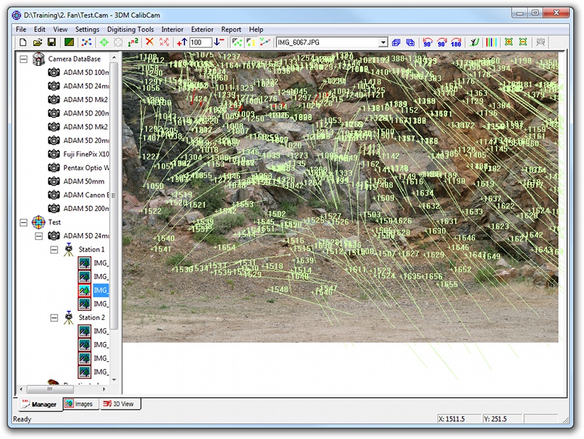
(Note that in the example image I had to reduce the residual scale from the default value of 100 × to 4 ×, because otherwise the residuals would be so big you couldn’t see the pattern. They are big!)
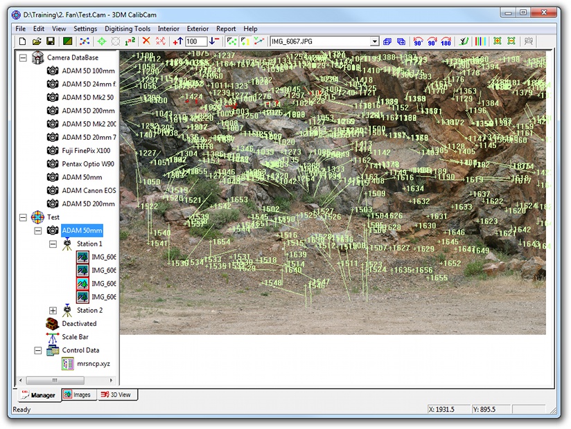
(Note that in this example image, the residual scale is at the default value of 100 × and the calibration is correct except for a 10% error in the focal length. The pattern is similar to above but the error is much smaller.)
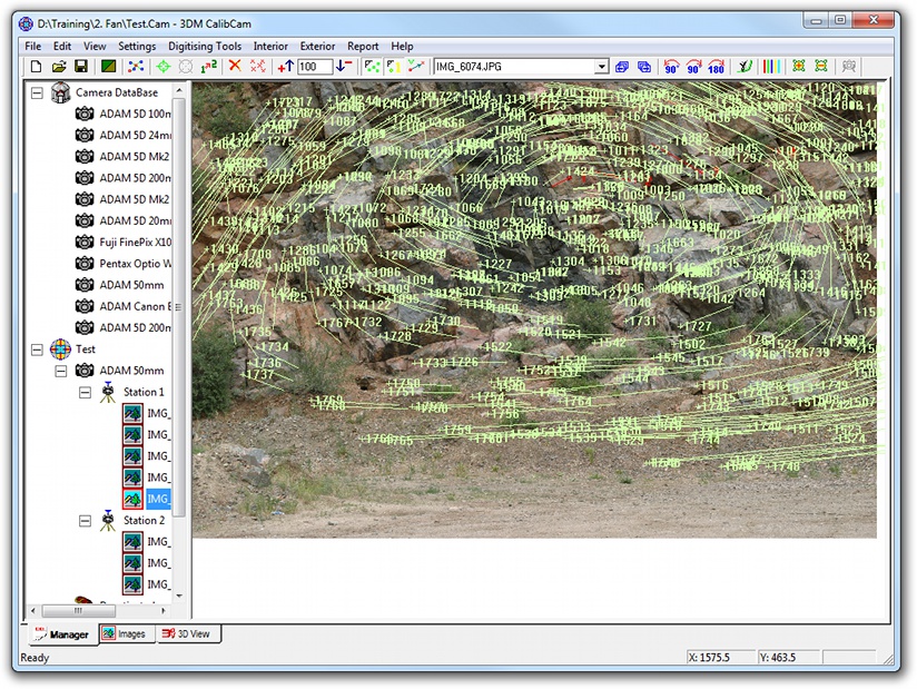
(Residual scale reduced to 10 × so the pattern is visible.)
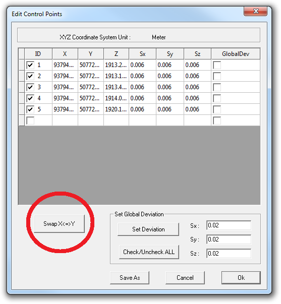
All of the above were systematic errors related to the images themselves, that will tend to show up in the image residuals regardless of whether a free network or control network exterior orientation is performed. However, the co-ordinate system itself is also a model — a right-handed Cartesian co-ordinate system, in fact. Right handed means that if you make an “L” shape with the thumb and first finger of your right hand, and poke your middle finger out so that it’s perpendicular to your palm, then your thumb represents the X axis, your first finger represents the Y axis, and the middle finger represents the Z axis. An example of a right-handed co-ordinate system is (East, North, Height). Surveyors very commonly report co-ordinates as (North, East, Height) instead, which is a left-handed co-ordinate system. Accidentally use these co-ordinates in your project and you will get very large residuals on your control points because, again, the model is wrong. Fortunately, because this is such a common problem, the software includes a handy button on the Control Points dialog that allows you to Swap X and Y:
3DM CalibCam is also very good at robustly detecting control point blunders with its “Troubleshooting” function. Blunders can either be because the control point data that was supplied was wrong, or because the control point was mis-identified consistently, or because the control point was mis-identified inconsistently. By “inconsistently” I mean the user picked up a control point in one image at a certain location, but picked up the same control point in a different image in a different location. The latter case will show up with large residuals for that point even in a free network adjustment, whereas the former two cases only show up when doing a control network, so it’s quick and easy to detect the last type of error. (The reason we now teach users to get a free network working first, then digitise the control points, then do the control network, is to make it more obvious what the source of the problem is. If everything was going fine until you added the control points then you know the control points are the source of the error. Additionally, the reason we now teach users to only digitise three control points to begin with, and use driveback for the rest, is because if something is wrong you’ve only got three points to check!)
Whew! If you’ve made it this far then I hope you have a far better appreciation for the value of residuals and a much better idea of how you can use them in practice to detect problems and solve them. I strongly recommend taking a good, working project, and deliberately introducing the various forms of errors I’ve identified above to see what the effect is — change a control point’s value, for example, or the focal length in the camera calibration, or use a different calibration altogether, or manually digitise some bad relative-only points.
One final note I’d like to make is this: when starting a camera calibration project for a new camera, of course the model is wrong! The parameters haven’t been determined yet — that’s why you’re calibrating it! So expect large residuals with systematic errors in them until you have actually performed the Interior Orientation. Be very wary of removing “bad” relative-only points, either by hand or automatically, because perfectly “good” points will have high residuals simply because the model is wrong.
Pingback: Aerial Mapping with UAVs and 3DM Analyst Mine Mapping Suite « ADAM Technology Team Blog